Understanding And Doing Better With SUMIF Function

SUMIF() functions is among the most commonly used functions in excel. Whenever ever we have to sum against a given criteria we revert to this function, be the criteria be only one or more then one (for more then one criteria’s we use SUMIFS(), just another function of this family).
The SUMIF() Family:
There are two variations of SUMIF():
-
For single criteria – we use SUMIF()
-
For multiple criteria’s – we use SUMIFS()
The formula’s syntax:
SUMIF(range, criteria, [sum_range])
SUMIFS(sum_range, criteria_range1, criteria1,[ criteria_range2, criteria2],…)
The range refers to the range of cell where we want to validate a criteria, and is equivalent to criteria range in the SUMIFS() formula. The criteria, refers to the condition that we want to validate over the range of cells. For SUMIFS() we can have multiple ranges and corresponding multiple criteria’s as well, but you can see from the large braces that the second range and criteria in the SUMIFS() is just an optional feature and can work without it as well.
In following paragraphs we will discuss few examples of using both of them with various conditions.
How to sum if cell contains text – single criteria:

Consider the example in the example sheet1 that aims to sum the score for all the contestants excluding blank cells in Column A. The target can be achieved with the use of following formula – parts of which are explained in following diagram:
Note that we use logical operators to express logical conditions – the symbol <> represents condition of “other then” and ampersand sign (&) is used to perform concatenation. The blank space is represented by “”. (Had we been interested in summing only blank cells, we would have used “=”&”” as our criteria.)
How to sum if cell contains text – single criteria:
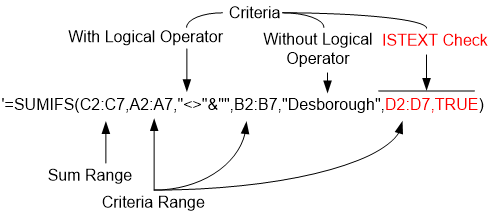
When we add more then one criteria, we have to revert to SUMIFS() that has provision to accommodate the change. The following diagram refers to the second example in the workbook (Sheet2). We have again used the logical operators, where required, and in the second criteria, we do not one.
In this example there are two criteria ranges and corresponding criteria as well. The summation range will remain only one. The formula will also work even if we omit the second criteria (as it is optional), but will sum based only on first criteria.

Checking if a cell contains text and summing a column:
The logical operators are used in our precious formulas if we wanted to check for blank cells. In case we are interested in summing for only that cell that is non-blank, the formula can be adjusted by adding an additional column. The column should contain formula: ISTEXT() that checks for text or non-text entries.

Thus adding a third criteria will resolve the issue and give us the result.
The main disadvantage of using SUMIF() family is that they can not be used as an array formula. That is the reason we have to add a column for ISTEXT() function. However SUMIF() formulas are faster then most of the custom produced array formulas.


