One of the most versatile and highly used functions is VLOOKUP. Whenever we have a table and want to quickly retrieve a value, we have to revert to VLOOKUP. Let’s take a quick dive into its use and how we can get maximum out of its use.

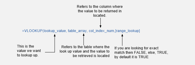
The VLOOKUP Syntax:

The formula uses four arguments, of which 3 are mandatory and the last one is optional. The function works by looking up for a criteria in a table and retrieving the corresponding value from the nth specified column, giving either exact or an approximate match for the criteria.

Here is an elaborated diagram for the function’s syntax.

Examples, Examples and Examples:

As has been our routine, we will take up few examples and see how the formula works out. Please refer to the sheet with this tutorial:

Example 1 – Retrieving the Exact Match:

A teacher is interested in finding the marks of one of his student from the Student Database in school. The IT Department provides him with an excel worksheet mentioning marks of all the students for a particular class for that year. Can you help him find the marks?

Yes! You can suggest him to use VLOOKUP – The formula (referring to the sheet1 in workbook) should look like this:

=VLOOKUP (E2,$A$1:$C$9,3,FALSE)

The syntax has already been explained. The criteria is located in cell E2, the table referred is located in cell $A$1:$C$9, 3 refers to the column offset (remember that column numbering always start from 1, 1 being the left most column), and FALSE for an exact match type.

The result is Reeta for this specific case.

A twist in VLOOKUP – Double LOOKUP with VLOOKUP:

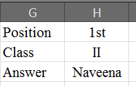
By now we just looked up for criteria in the left most column of the table. But now the teacher is in retrieving the name of the student who secured 1^st position from a class. The IT department has again provided his with a table that looks like following:

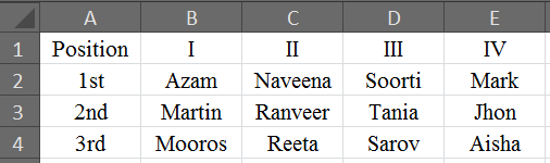
The teacher now needs to look up at both left most column as well as the top most row, whereas the VLOOKUP() formula can only look at the left most column! In order to make a formula that is robust enough to meet the requirement we need to introduce a MATCH () function within VLOOKUP () syntax so that we do not need to do this match-process manually.

Here is the formula that will work:

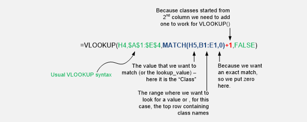
The MATCH () function has been discussed in our previous post, here the use of this formula ensure that we don’t need to change the 3^rd argument of VLOOKUP every time we want to change the class. Thus with a simple tweaking of formula, we can automate this stuff.

You can still create variation of the VLOOKUP – MATCH combination, we can add multiple criteria’s and lookup ranges by concatenating them using ampersand sign (“&”), or simply add column index numbers, in case columns are not sorted, to make VLOOKUP to lookup into any specific column, as our need.

I hope you have found this tutorial useful. In our next post we will revert with some other function and its unique usage.