The MATCH function of Excel 2016 permits users to select the position of an object in a range instead of selecting the entire actual item. This can prove to be extremely useful, for example, when you are in need of the “row_num” parameter while using the INDEX function. This function has three significant arguments in its syntax. The syntax of the function is:

MATCH(lookup_value, lookup_array, [match_type])

The first parameter is concerned with the value of the object you are looking for; lookup_value. The second parameter, lookup_array, deals with the range you would like to make your search in. The third parameter is restricted to 1, 0, or -1, based on the kind of MATCH you are looking for.

How to Use Match

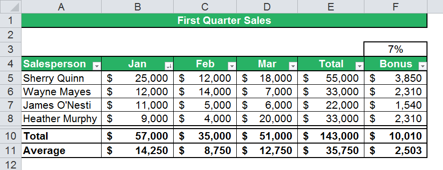
The first example to show how to use MATCH comprises of first quarter sales for a group of sales persons.

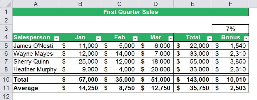
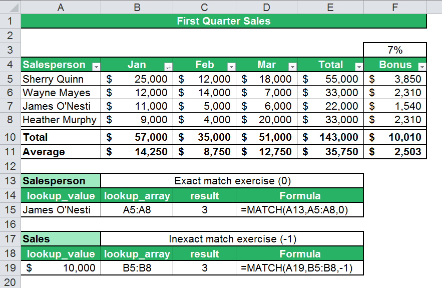
We will first try to locate an exact MATCH for “James O’Nesti”. When you are trying to find a MATCH, you must keep in mind that the function will only provide you with the relative location of the name in the table. For example, if James O’Nesti’s name is in row 5 in the worksheet and our “lookup_array” is A5:A8, then the outcome of our MATCH would result in “1” because the relative location of our search up value is within that particular range.

Inexact MATCH with match_type

You can easily use 0 as a match_type for an exact match, but what would you do in the face of inexact MATCH values of 1 and -1?

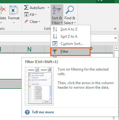
For example, if you wanted to find the sales total greater than an amount of ten thousand dollars for January, you would want to utilize the inexact MATCH -1 function because this will search up the smaller values that are equal to or greater than the “lookup_value”. In order for the inexact MATCH -1 parameter to operate properly, you must ensure that you are sorting your lookup_array values from largest to smallest. You will need to highlight the row that has all the table headers by selecting the row numbers all the way to the end of the row. You must then make your way to the Editing area and select “Sort & Filter” and choose “Filter” from the dropdown list that appears.

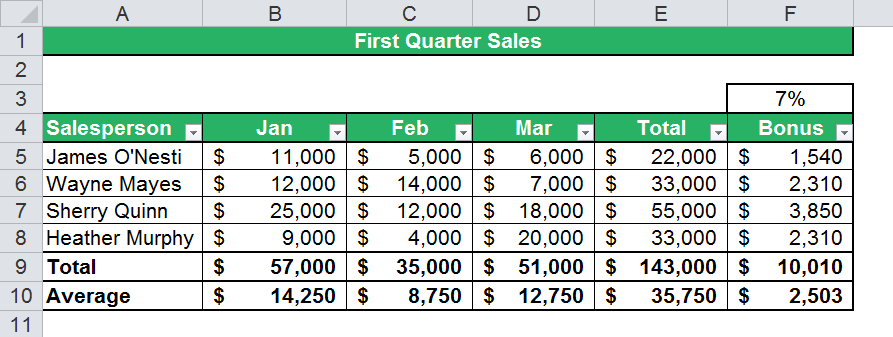
Once you have done that, you will notice that filters will become activated at the column headers as shown below:

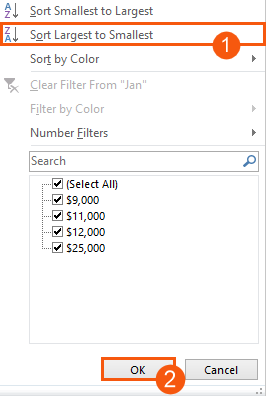
You can now set the settings to “Sort Largest to Smallest” from the drop down list that appears when you click on the arrow and click on OK to begin arranging the values.

You table is now set in proper order and you can now rest assured that your MATCH function will operate the way it is supposed to when making the search.

You could type in ‘=MATCH(10000,B5:B8,-1)’ to get the desired result, but you must keep in mind that you should not put commas to separate the thousands, because Excel will assume that you are inserting another argument rather than separating the thousands.

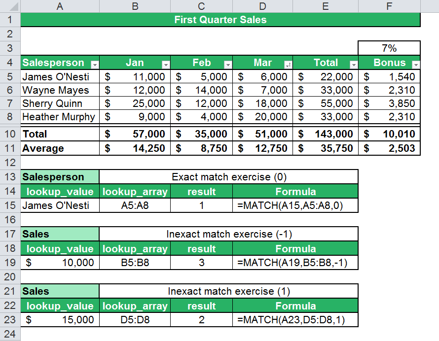
Our result for this search will be “3” because the smallest amount of sales that are greater than $10,000 is $11,000, which is the third value on the list.

Inexact MATCH and match_type 1

Rather than using the -1 match_type parameter, let’s consider a different cutoff sales value of $15,000. This will require you to set your sales column ascending order for the MATCH function to operate properly. The formula will look like:  ‘=MATCH(A23,D9:D12,1)’. The result is “2”, which basically means that every value that is above the second position on the table is a number less than fifteen thousand dollars.