Understanding How HYPERLINK Works In Excel

Excel has a built in function to create hyperlinks – named �HYPERLINK�(). This function is useful when you want the user to be redirected to some other place for example a webpage or a document or some place within the excel sheet.
In today’s post we will understand the syntax and the usage of �HYPERLINK�() function with some useful and practical examples.
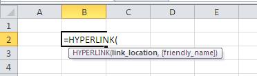
The Syntax:
The �HYPERLINK�() function takes two arguments:
-
The Link_location – or where you want to redirect the user.
-
Friendly_name – that is an optional argument to name the link.
The user can skip the second argument that is optional but it is better and sometimes more aesthetically appealing to use it. You can use it cover long and complicated urls with a small word or phrase.
Examples:
The syntax of the function is not that complicated, we will try to elaborate the use with following examples:
Example # 01 – linking to a cell within sheet:
User can create a hyperlink referring to cell within sheet – when a user will click it, will be directed to that cell. Use following formula:
=�HYPERLINK�("[Example_Hyperlink.xlsx]a1", "Click Here")
Note that we need to fully qualify the address of the cell otherwise formula would not work.
Example # 02 – linking to a cell to some sheet with location (drive) specified:
A user can link to some other sheet as well and will be required to qualify the drive where the file is present. In such case the formula will take the following shape.
Drive_name:\Parent_Folder\Sub_folder\another_subfolder\name_of_sheet.xlsx
Following by the data to be displayed from the cell (for example) in A1.
The final formula will be of the following form (assuming our file was present in E drive)
=�HYPERLINK�("E:\Sheet_Zoom\MyExample.xlsx", A1)
Example # 03 – linking to named ranges in different sheets:
If you have named range in another sheet – say “myscore” then you can link it to the a cell in you active sheet with this formula:
=�HYPERLINK�("[E:\Sheet_Zoom\MyExample.xlsx]myscore")
Example # 04 – Hyperlinking to a webpage:
We can hyperlink to a webpage with HYPERLINK function in the following way:
-
Assuming that the link in present in cell Al, the hyperlink can be created with the following formula:
=�HYPERLINK�("https://www.google.com.pk/", "Google It!")
-
Alternatively you can put the link in the cell and then use a HYPERLINK function:
=�HYPERLINK�(A1, "Google It!")
We have assumed that link is present in cell A1.
Example # 05 – Jumping to a place in Word Document:
We can created a link that is directed to a word document – this is done by using hyperlink function, directing it to the word document and by making use of the BOOKMARK tool in the word document and referring to it in excel sheet.
=�HYPERLINK�("[myexample.docx]myscore", "myscore")
Conclusion:
Hyperlinks can be created by using the menu bar or by using a formula. These are handy when you want to direct user to a different place within sheet or outside of it. The important point is that the address need to be explicitly and fully qualified for a hyperlink to work.

Related Tutorials
We encounter this problem of numbers behaving as text with commas when we import data from some other software in to excel sheet.
.png)
If you have a large pivot and want to create a report based on that pivot, it is time to revert to a function dedicated for it – GETPIVOTDATA().

There are times when you bring data from other software to excel sheets and find that some of the numbers are formatted as text


Latest
-
Understanding How HYPERLINK Works In Excel
Excel has a built in function to create hyperlinks &...
-
Understanding how MS Excel Query Works
“Query” in MS Excel has same meaning as ...
-
An Introduction To Excel Power Map
Our today’s post is about “Power Map&rdq...
-
Using Pivot Charts For Displaying Data
Conventional charts are mostly used for displaying r...
-
Using “Calculated Items” For Analyzing A Pivot Table
In our last post, we explored how to use calculated ...