Using Index-Match Combination To Ease Up Lookup Process

Most of the time when we are stuck with lookup and return something process, we revert to VLOOKUP() and occasionally HLOOKUP(), according to the situation. The same process can be achieved by using combination of two excel functions – MATCH() and INDEX().
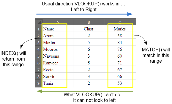
One may ask why this combination when we already have a dedicated formula? Answer - VLOOKUP() can not look to the left of the lookup value. The left most column is the column from where VLOOKUP() starts and keep going right-wards, but nothing to the left is allowed.
At this point, the MATCH-INDEX combination jumps in. This combination gives you the freedom of matching in any column or row and then indexing and retrieving from any where from the table, be it on right, left, top or bottom. Remember that VLOOKUP() only works for columns and if you are looking in rows, you have to use HLOOKUP().
So this provides a robust and generalized solution to the problem – let your lookup value be any where in the data as well as the value you want to retrieve, it will work, if the length of arrays don’t match, it will give you an error.
So lets take these functions one by one and see with examples, how they work.
The MATCH() function:
The MATCH() function matches a given criteria to a range of values for exact or approximate match. The syntax for the function is =MATCH(lookup_value, lookup_array, [match_type]). If you choose to omit the last option, the function will fetch the approximate match.
The INDEX function:
This function return required indexed item from an array. It works two ways – first by taking an array and then returning the result and secondly by taking a reference and then working out details to fetch the result. We will be using the first syntax for now and that is =INDEX(array, row_num, [column_num])
The Simplest Example – replicating VLOOKUP
Referring to the Sheet1 attached with this tutorial, this is the same data table we used while learning VLOOKUP(). The entire process can be repeated for the same result using MATCH()-INDEX() combination with the following formula:
=INDEX(C2:C9,MATCH(E2,A2:A9,0))
The formula yields the same result as done by VLOOKUP. The syntax has already been explained in preceding lines. Here the MATCH() function forms the second argument of the INDEX() function, where zero in the last argument of MATCH() ensures exact match.
Looking to the left side – Overcoming VLOOKUP’S shortcoming:
Referring to the same table, what if we wanted to know the name of the student provided marks obtained by him are given as match criteria.
The solution will involve simply referring to the required range on the right side with INDEX() function so that data can be retrieved from it.
Not only this, MATCH()-INDEX() will also work for rows as well, the indexed range could be a row and the data can be retrieved from it as well.
This is all about INDEX & MATCH combination.

Related Tutorials

One of the most versatile and highly used functions is VLOOKUP. Whenever we have a table and want to quickly retrieve a value, we have to revert to VLOOKUP. Let’...

We came across such situation we have multiple choices and we want to find the best possible combination of them, be it spending money on shopping or adopting a route ...

Two dimensional lookup is obvious – we have a header row and a column and we want to look at the intersection of the two criteria’s.


Latest
-
Understanding How HYPERLINK Works In Excel
Excel has a built in function to create hyperlinks &...
-
Understanding how MS Excel Query Works
“Query” in MS Excel has same meaning as ...
-
An Introduction To Excel Power Map
Our today’s post is about “Power Map&rdq...
-
Using Pivot Charts For Displaying Data
Conventional charts are mostly used for displaying r...
-
Using “Calculated Items” For Analyzing A Pivot Table
In our last post, we explored how to use calculated ...