Performing The Three Dimensional Lookup

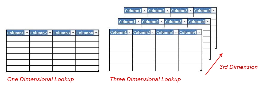
Two dimensional lookup is obvious – we have a header row and a column and we want to look at the intersection of the two criteria’s. But what about three dimensional lookup? The third dimension of the lookup is added by adding third characteristics to our lookup – i.e. tables. When we do simple two dimensional lookup we are actually working on a single table, but when we go for three dimensions we have number of tables in line for a particular search.
In this post we will try to learn how to do a 3-dimensional lookup.
As usual we will start with an example. Consider a case where we have workbooks with three similar worksheets, each representing a month. The specifications of the table are same i.e. they same number of rows and column.
A three dimensional lookup will perform lookup based on three criteria’s:
-
The criteria for header row
-
The criteria for header column
-
The criteria for the table
With all this information we will try to setup a solution that can give us the result of such a search.
Step # 01 – setting up formula for two dimensional lookup.
First, we will setup the formula for two dimensional lookup. The formula that we will use is �VLOOKUP�() and �MATCH�(). The �VLOOKUP�() is used to perform the lookup, and the match is used to set the column index.
The formula becomes:
=�VLOOKUP�(D3,Jan!$B$3:$E$9,�MATCH�(LookupSheet!D4,Jan!C3:E3,0)+1,0)
Within this formula, the �MATCH�() function is serving the third argument that looks for the column offset. And since we want to skip the first column that is header column, we have added one to the result of �MATCH�() function.
The final formula works this way: look for the value in cell D3, in the range Jan!B3:E9, with column offset that we get as a result of �MATCH�(). The �MATCH�() function works by looking in the range Jan!C3:E3 for value D4, with an exact match criteria and 1 is added to the result to adjust for the first header column. The �VLOOKUP�() returns the result also for the exact match.
Step # 02 – adding the third dimension:
If we look at the following formula the points that refer to the worksheet are actually the name of month. These of month in following figure are marked with red colored line.

If somehow we are able to change this month, we can select the table to perform the lookup. This will actually add the third dimension or the ability to perform the lookup across the workbook.
In order to do this, we will need help from a third function called the �INDIRECT�() function. The formula that will work for setting up the table reference will be:
�INDIRECT�("'"&D5&"'!"&$F3)
Here D5 contains the Sheet name and the F3 contains the range entered in the cell. The content of the formula will eventually evaluate to:
‘Jan! $B$3:$E$9
That will be the part of the of second argument of VLOOKUP. The next fix we need to set the lookup range for the header row – for our case it is C3:E3. The formula with INDIRECT () will be:
�INDIRECT�("'"&D5&"'!"&$F4)
And it will evaluate to following:
‘Jan! $C$3:$E$3
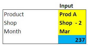
With all these sub sections of formulas, the formula will evaluate and will return the result when we will change the worksheet name. The final output looks like this:

Related Tutorials

We came across situation we have to look for values both horizontally and vertically.
.png)
Using ROW() and COLUMN() functions.
Whenever we have data, we want to extract meaningful information from it.


Latest
-
Understanding How HYPERLINK Works In Excel
Excel has a built in function to create hyperlinks &...
-
Understanding how MS Excel Query Works
“Query” in MS Excel has same meaning as ...
-
An Introduction To Excel Power Map
Our today’s post is about “Power Map&rdq...
-
Using Pivot Charts For Displaying Data
Conventional charts are mostly used for displaying r...
-
Using “Calculated Items” For Analyzing A Pivot Table
In our last post, we explored how to use calculated ...