The up and down arrows on stock exchange information board is the life line of trading business. The information displayed is designed to guide traders with spontaneous and the most relevant information and the fact remains that humans can understand symbols and picture more readily then written text. The fact has lead to the use of graphs, symbols, spark lines and much more to make the process easier.

And it is not just stock exchange that uses tickers; any performance dashboard can have it. Even if you are monitoring on daily basis and you wan to see if the parameter has improved or not, you can have ticker for it. 

There are two ways to create it: one is by using Conditional Formatting Icon Sets and the second one is by using Symbols with different fonts.

Let’s take them one by one and see how we can do it.

Creating Tickers with Icon Sets:

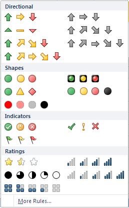
The icon set in conditional formatting can be accessed through Home>Conditional Formatting>Icon Sets>Directional (in Excel 2010) and looks like the picture on the right side.

Simply select the cell where you want to apply the formatting. The cell will start display the three arrow heads, based on the value of the cell, once we are done with it.

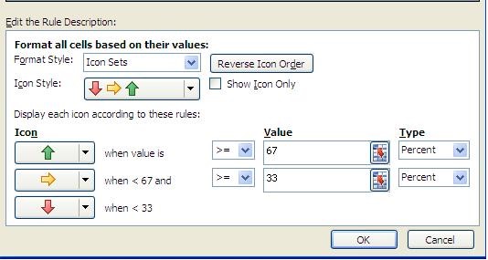
The rule based on which the arrows are changed can be set by right clicking the cell Conditional Formatting > Manage Rule > Edit Rule that allows you to edit the conditions. With three-arrow set you have 02 rules that can be used to set the three steps.

Green forms the top most groups, referring to the picture, on right, when the value in greater then or equal to 67% , yellow for values between 33% and 67% and red for less then 33% of the minimum value. The formula for calculating these arbitrary percentile values is:

%Value = Min + Range × %age

You can also change the setting to put up absolute values to format the arrows.

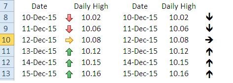
Referring to the example sheet, the max value is 10.16, min is 10.02 and range is 10.12 for 67% mark, thus all values greater then 67% will be marked green. Similar all values between  10.07 and 10.12 will be yellow directional and all the values below 10.07 will be red.

 Creating Tickers with Symbol Fonts:

We can Windings Font for producing arrows. With Wingdings, Character 223 to 248 produces different types of arrow heads that can be used with formulas to give desired results. You can use following table coupled with IF() formula to get the results:

Referring to the example sheet, you can use the following formula to get similar results:

=IF(B8<=$B$4,CHAR(234),IF(AND(B8>$B$4,B8<=$B$5),CHAR(233),CHAR(232)))

The formula uses three nested IF() that check for the range in which the value falls and return the corresponding character. The character is then formatted using the Wingdings font giving the desired result.

Thus we have produced almost the same results that we produced with Conditional formatting icon sets. The idea of using fonts is appealing because we can use a lot different types of symbols with this technique.