Using Excel’s Multiple Criteria In VLOOKUP Function
.png "Using Excel’s Multiple Criteria In VLOOKUP Function")
Microsoft Excel’s VLOOKUP function is a popular feature amongst office personnel and data processor positions. Those users who already have an advance understanding of this function have utilized it by putting an additional criterion for search purposes.
The default characteristic of the VLOOKUP function is that it cannot have a lookup with two or more criteria. Most people use it with a combination of other functions such as Match and Index to deliver desired results.
In the following example, steps on customizing a VLOOKUP function with multiple criteria are discussed. The demonstrations are done using Microsoft Excel 2016 (Windows) but the general concept can be used universally across other versions of the program.
Main Concept
To do this multiple criteria VLOOKUP, all the desired criteria must be compressed into the main function. Using the ampersand (&) symbol, we can input all the criteria within the syntax. In line with this, we will need to join the ‘Table_arrays’ by creating a helper column.
Helper Column
For this demonstration, we will create a distinct column to combine the data in the Employee and Department columns. Insert a new column after B and name it as defined by your purpose in cell C1. Input =A2&B2 into cell C2 and copy this to all the succeeding cells.
VLOOKUP Syntax
When inputting the =VLOOKUP, Excel will display the needed values you will need to supply for the function to perform accurately. These are: ‘lookup_value’, ‘table_array’, ‘col_index_number’ and [range_lookup].
The Lookup Value
The last detail in this multi-criteria VLOOKUP is to edit the function’s lookup value. It must be the combined criteria you would like to incorporate in the function. For this example, we will put the formula in Cell F2, the first and second criteria in cells G2 and H2 respectively. The resulting input should now be G2&H2
That’s it!
The above steps are the plain gist of the process. You can now use this method for yourself and try it out on different purposes.
VLOOKUP With Multiple Criteria Example
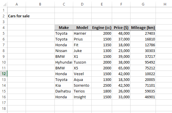
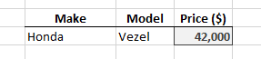
1 - Let’s consider that we have a data table of a car sale and we want to look up some data with multiple criteria.
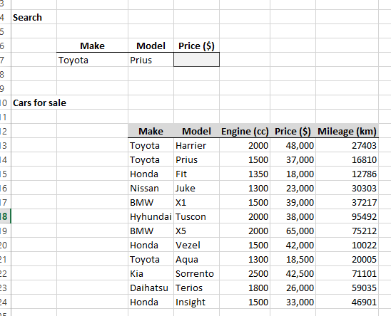
2 - We want to retrieve the price of a car using car make and model. Note that the car make and model are in columns. For this we can make a simple table to retrieve the required information.
3 - We are using the traditional lookup function (VLOOKUP) along with the CONCATENATE function. So we have to first create a single lookup column first.
This can be easily done with following CONCATENATE Syntax, as shown below. Which combines cells C13 and D13.
=�CONCATENATE�(C13,D13)
The new lookup column is illustrated in the first column below:
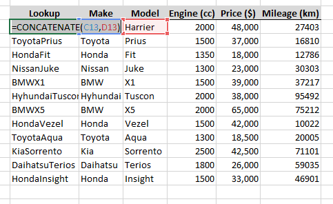
The Lookup column joins values from C and D columns that are used as criteria. It must be the first column of the data table, and functions as the key column for LOOKUP function.
lookup_value:
Lookup value is set as B7 & C7, which are the make and model of car.
table_array:
Set up a VLOOKUP formula that refers to a table that includes the helper column. The helper column must be the first column in the table.
col_index_num:
The column number of the retrieving data is no.5 (i.e. Price $).
range_lookup:
Since we want to retrieve the exact match, False is given as the range_lookup
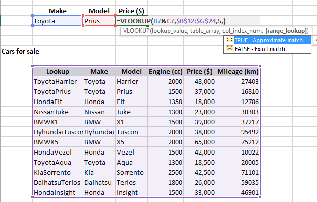
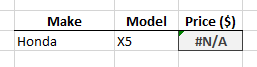
5 - Now the function is set to retrieve data from the table.
If the data retrieving cannot be accomplish for the given Make and Model, the result will be given as N/A.

Related Tutorials

There several ways to create in cell and that includes Excel’s built in Sparklines or using a third party Sparkline Add in, But there are ways to produce bar cha...

Data bars are amongst one of the many feature excel has for presenting data.

Microsoft Excel 2016 introduces a lot of new Charts for us to use in presentations.


Latest
-
Understanding How HYPERLINK Works In Excel
Excel has a built in function to create hyperlinks &...
-
Understanding how MS Excel Query Works
“Query” in MS Excel has same meaning as ...
-
An Introduction To Excel Power Map
Our today’s post is about “Power Map&rdq...
-
Using Pivot Charts For Displaying Data
Conventional charts are mostly used for displaying r...
-
Using “Calculated Items” For Analyzing A Pivot Table
In our last post, we explored how to use calculated ...