There several ways to create in cell and that includes Excel’s built in Sparklines or using a third party Sparkline Add in, But there are ways to produce bar charts by using Excel without using these feature. This small tutorial will show you how to create one by using the Font type Symbols and using excel formulas.

The advantage of using such a method is that it makes sharing and excel file easy and the recipient does not need to have same add in or version of Excel.  So let’s jump start with how to make such graph.

Procedure:

Put your data in appropriate range:

The charts works best when done along-side of the data. So spare some space on the side (preferably right side) of the data.

Get familiar with the REPT() function:

The REPT() function can repeat the given character specified number of times. Thus if you put REPT(“*”,3) you will get “***” as result. In order to create bars, we will be using this formula.

Setup the symbol you will be using: 

There are several symbols that can be used to produce a bar chart. The best one is to use a filled box with the font web dings and the character “g”. This produces a smooth filled box like this: g. Alternatively you can also use any of the following symbols:

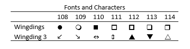
To use these symbols simply use formula =CHAR(any_symbol)

Putting all things together to get the chart

The final arrangement should look like this one:  The font is set to Webdings and the cell C3 contains the formula: =REPT(“B3”,”g”) where B3 contains the repeat frequency.

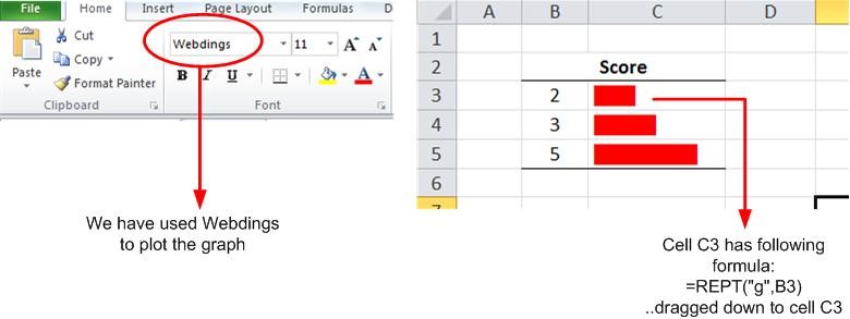
With this setup you can easily produce bar charts that are independent of any add-in and will work even on Excel 2003 and 2007.