How to Use Sumif

The SUMIF function is used to conditionally sum values based on a single criteria.
The Syntax of this SUMIF function can be explained as follows:
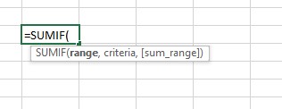
=SUMIF(range, criteria [sum_range])
Here, ‘range’ refers to the cells that you want to be analyzed by the ‘criteria’.
‘criteria’ refers to the condition that specifies which items are to be added. ‘criteria’ can be a number, expression or a text string.
‘sum_range’ is an optional argument, it specifies the cells to be added. If ‘sum_range’ argument is omitted then SUMIF treats ‘range’ as ‘sum_range’.
Simple worked example
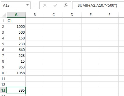
For instance, if you want to sum the numbers that are larger less than 500. You can use this function with the following simple formula: =SUMIF(A2:A10,"<500")
This can be used in different ways to suit the requirements in day to day and professional uses.
Example 2
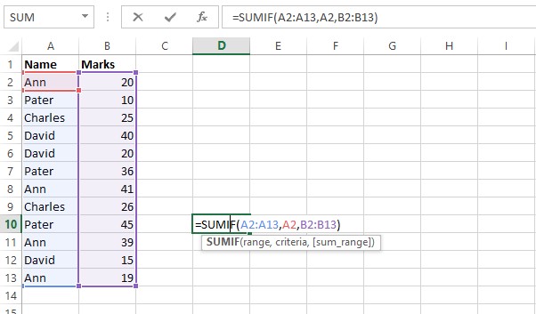
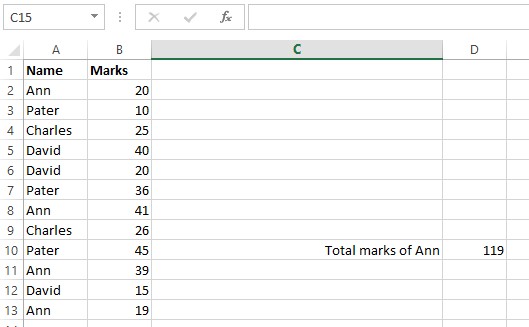
Let’s think that we want to sum marks of Ann from the marks table shown above.
Range:
The first parameter in the SUMIF function is the range of cells that you want to apply the criteria against.
In this example, the first parameter or the range is A2:A13. This is the range of cells or the names of students that will be evaluated to determine if they meet the criteria.
Criteria:
The second parameter or criteria in the SUMIF function is the name of student we want (i.e. Ann) that will be applied against the range, A2:A13.
In this example, the criteria is A2, which contains the name Ann. This is a reference to the cell A2 which contains the text ‘Ann’. The SUMIF function will test each value in A2:A13 to see if it match with Ann.
Sum_range:
The third parameter in the SUMIF function is the range of numbers that will be summed together.
In the above shown example, the third parameter is B2:B13. For every value in A2:A13 that matches A2, the corresponding value in B2:B13 will be summed.

Related Tutorials
.png)
The SUMIF function is used to conditionally sum values based on a single criteria. The Syntax of this SUMIF function can be explained as follows:

The SUMIF function is used to conditionally sum values based on certain criteria. Another version of that function is SUMIFS
.png)
The COUNTIFS() function is an extended version of the COUNTIF() function which is used to conditionally count items/ cells based on certain criteria.


Latest
-
Understanding How HYPERLINK Works In Excel
Excel has a built in function to create hyperlinks &...
-
Understanding how MS Excel Query Works
“Query” in MS Excel has same meaning as ...
-
An Introduction To Excel Power Map
Our today’s post is about “Power Map&rdq...
-
Using Pivot Charts For Displaying Data
Conventional charts are mostly used for displaying r...
-
Using “Calculated Items” For Analyzing A Pivot Table
In our last post, we explored how to use calculated ...