The SUMIF function is used to conditionally sum values based on certain criteria. Another version of that function is SUMIFS what we explain now, is used for multiple criteria purposes.

The Syntax of this SUMIFS function can be explained as follows which is similar and as simple as SUMIF function syntax:

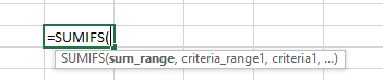
=SUMIF(range, criteria_range1, criteria 1, criteria_range2, criteria 2…..)

Here, ‘range’ refers to the cells that you want to be summed by satisfying the number of conditions or criteria.

‘criteria 1’ refers to the first condition that specifies which items are to be added. ‘criteria_range1’ refers to the cell data range of criteria 1.

Similarly, multiple conditions can be added to criteria_range2, criteria 2…..

Note: Criteria can be a number, expression or a text string

Example

Consider the following data set that shows car stock availability based on car manufacturer, engine capacity and price. We want to find the number of available cars based on each factor using conditional arguments.

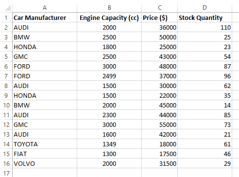
If we want to find number of AUDI cars at stock which have engine capacity less than or equal to 2500cc and which are priced less than 40000$, then the ideal method is to use SUMIFS function.

There are three conditions:

• Car Manufacturer:                AUDI

• Engine Capacity:                    Less than or equal 2500cc

• Price:                                      Less than 40000$

he

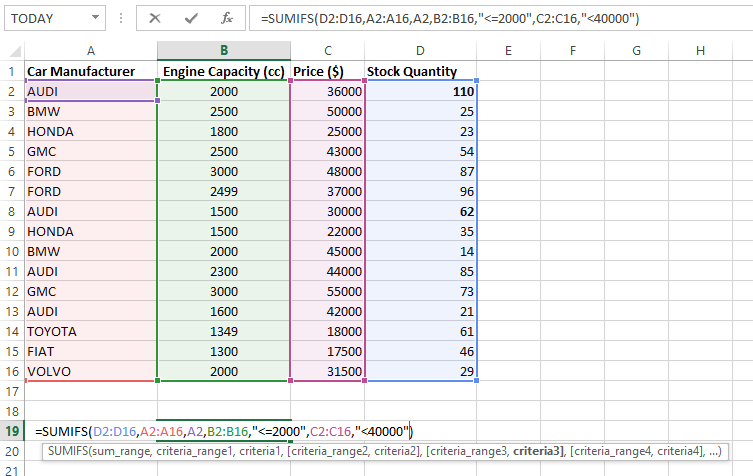
Those conditions are arranged in the following syntax.

=SUMIFS(D2:D16,A2:A16,A2,B2:B16,"<=2000",C2:C16,"<40000")

As you'll see, D2:D16 shows the available car stock. A2:A16 is the criteria 1 range and A2 is the criteria 1. B2:B16 is the criteria 2 range and “<=2000” is the criteria 2. Similar syntax is used for criteria 3.

Note that criteria 2 and 3 are included in double quotations.

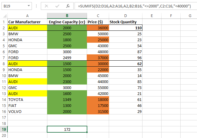
In the following snapshot, it shows the cells that satisfy all three conditions are summed for getting the answer (cell B19).