How To Use MOD() Function To Repeat Values Certain Number Of Time
 Function To Repeat Values Certain Number Of Time.png "How To Use MOD() Function To Repeat Values Certain Number Of Time")
MOD() function has variety of uses. One of the most basic one is that it is used to find the remainder from a division. Just to illustrate if we divide 5 by 2, we will have 1 as a remainder. The formula uses the syntax =MOD(number, divisor).
In this post we will see how we can create number patterns that repeat their selves with this formula. For example in the following picture, A is repeated at an interval of 6. We will learn how we can do it.

Doing this manually for large repeats would be troublesome. For this case, we will be using the COLUMN() function (since our data is positioned in a row).
Let’s see how we should proceed.
SET A HELPER ROW
Since our data is in a row, we will add a helper row. This helper row will contain a formula that will check the remainder from the division of column number with the repeat. The row will be followed by another row that will check if the column number divided by the repeat is what we are looking for. The entire setup looks like following picture

The column row uses the formula: =COLUMN() to give the current’s column’s number.
The Remainder row used formula: =MOD(A4,$D$1) to give remainder.
After setting up these two rows, we can put an IF() in action to see where we need to repeat the next. The logic works this way –if the value in the remainder row is zero, I will A to appear in the cell just below it”. Now this could be achieved using …
=IF(A5=1,"A","")
…simply checking if the value is 1 or not. All this results in the following pattern:

The combined formula for the case is =IF(MOD(COLUMN(),$D$1)=1,"A","")
ANOTHER VARIATION TO REPEAT A CHARACTER MULTLIPLE TIMES:
Another variation could be this type of repeat:

We will go in a similar way as we have done earlier. We will setup a helper row that will mention the column number and another one following it to divide the column number with the desired repeat.

In next step we will add yet another row to roundup values to the nearest digit.

The roundup formula used for this case is: =ROUNDUP(A4/$D$1,0)
As a last step we will setup a Lookup Table that will have all the desired value we want to fetch according to the rounded up values. The table looks like following:
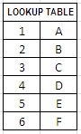
In another row we will add the formula: =VLOOKUP(A6,$H$11:$I$16,2,0) and drag to right to get us the final answer like following:

All these steps can be accommodated into the following single formula:
=VLOOKUP(ROUNDUP(COLUMN()/$D$1,0),$H$11:$I$16,2,0)

Related Tutorials

SUMIF() functions is among the most commonly used functions in excel. Whenever ever we have to sum against a given criteria we revert to this function, be the criteria...

The relationship listbox template has been used exactly zero times. One can build their classes from start along with names which actually reflect the objects of the b...
MS Excel has been used in many diversified areas; one of them is accounts and finance.


Latest
-
Understanding How HYPERLINK Works In Excel
Excel has a built in function to create hyperlinks &...
-
Understanding how MS Excel Query Works
“Query” in MS Excel has same meaning as ...
-
An Introduction To Excel Power Map
Our today’s post is about “Power Map&rdq...
-
Using Pivot Charts For Displaying Data
Conventional charts are mostly used for displaying r...
-
Using “Calculated Items” For Analyzing A Pivot Table
In our last post, we explored how to use calculated ...