MS Excel has been used in many diversified areas; one of them is accounts and finance. This sector of our lives uses it for variety of uses including book keeping, preparing various statements, analyzing scenarios and planning for the future needs of finance for the firms. It has been extensively used all levels of management within an organization and has become a standard practice to be used.

Amongst one of its uses in accounts and finance, one essential calculation is the use of spreadsheets for Tax Management and its calculation. This is often called tier based calculation where rates are changing as the tier or the level of income is changing.  The rates are often quoted as Slab Rates because they changes from one level to another.

A Tax Table has various classes for incomes tax and marginal tax rate column on the left. Following is an excerpt from the US Tax Tables for Singles for year 2017. (Source Wikipedia)

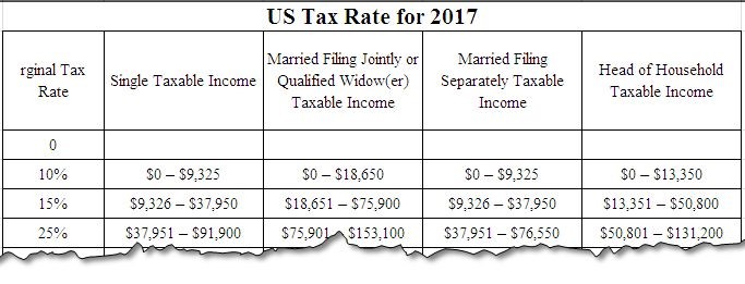
In order to automate the process we will be using once again VLOOKUP (), all other things being kept the same, we will be manipulating the last optional argument that states that should an exact match be returned or not. That will be the most critical point in this tutorial to understand.

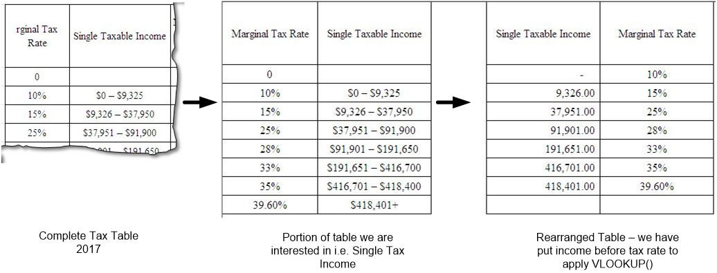
Before we proceed with the formula, we need some tweaking with the Tax Table.

For our VLOOKUP to work, we need to have the income bracket on the left most side, because it will be the value we will be looking for and tax rate on the right side (for this example we are only considering Single Taxable Income)  Thus following changes are needed.

You can see in the following picture how we have manipulated the data. One important point is how we have adjusted the slabs for tax rate.

In our newly formatted table, we have put the upper limit of the next slab as the threshold point to identify where the current slab is ending. This is because the formula will be looking up for an exact match or for the largest value smaller then the exact match.

The formula:

The formula we will be using is:

=IF(D11=0,0,VLOOKUP(D11,D2:E9,2,TRUE))

With values to be entered in D11. The VLOOKUP is nested in IF() as if some one enters zero, it will return a value error. The formula essentially looks for the value in D11 in the table spanned from D2:E9 and in the second column, with approximate match – and if found returns the value. In case the formula does not found an exact match the largest value smaller then the criteria is returned. If the user enters zero in D11, the formula returns a value error and the IF() function returns a zero.

Thus with a little effort, we can automate the process of tax rate calculation. We can do this for all the categories of income in tax table, and even make a formula to automatically pick up the category – this is left to you as an exercise (Hint: you need to use MATCH() to match categories along with  data validation.).

That is all for this post, we will return to you with some new topic soon. Take care.