Normally, the VLOOKUP function lookup function is normally not sensitive to case. For instance, the lookup function will treat Matt, matt and MATT lookup values in a similar manner. The first value that matches will be returned without considering case.

Creating a case sensitive VLOOKUP

If you have this set of data

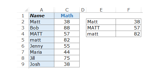
It could be seen above that there are 3 different names with different cases. When you search for matt, irrespective of the case you use the search, the first matt on the list will always come up.

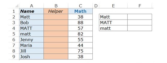
How to use helper column to make a case sensitive VLOOKUP

It is possible to get a lookup value that is unique for every item in the array for lookup. This results in a differentiation between the case for letter names.

• Put Helper Column at the column left, based on the location you intend for data to be fetched.

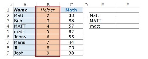
• Use the =ROW() formula so that every cell will have the number for the rows

Explanation of the formula

• EXACT(E2,$A$2:$A$9) equates the particular look value with other values on the column. It them returns false when there is no match and true when there is an exact match.

• EXACT(E2,$A$2:$A$9)*(ROW($A$2:$A$9) displays the row number when there is an exact match and a 0 where there is no exact match.

• MAX(EXACT(E2,$A$2:$A$9)*(ROW($A$2:$A$9))) gives the highest value from the number arrays.

There is however another alternative if you do not want to use the helper column

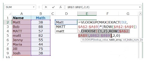
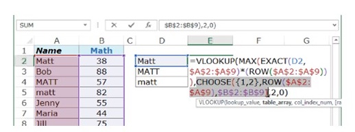
Creating the case sensitive VLOOKUP without using helper column.

Even when you do not want the helper column, you might still require virtual helper column.

The formula to be used include:

=VLOOKUP(MAX(EXACT(D2,$A$2:$A$9)*(ROW($A$2:$A$9))),CHOOSE((1,2),ROW($A$2:$A$9),$B$2:$B$9),2,0)

The workings of the formula

The helper column concept is also required by this formula. The only thing that distinguishes this formula is the fact that the worksheet does not need a helper column, it is however still there in a virtual form. The bolded part of the formula is similar to helper data.

=VLOOKUP(MAX(EXACT(D2,$A$2:$A$9)*(ROW($A$2:$A$9))),CHOOSE((1,2),ROW($A$2:$A$9),$B$2:$B$9),2,0)

The picture below shows the virtual helper data.

From this, pressing F9 after selecting the above will give the result below

The result above is an array and same row cell is represented with a comma while the next row is represented by a semicolon.

Applying the VLOOKUP formula checks the first column’s lookup value virtually and gives the score that corresponds with it. The value for lookup in this case is the no that is gotten from combining EXACT and MAX function.