In business, several tools are used to analyze data. One of such tools is the histogram. The histogram is a chart, which has chart columns that signify how frequent a variable is present. For instance, the histogram can be used to represent the frequency of staffs that has range of salaries such as 21,000 to 30,000, 31,000 to 40,000, etc.

Installing the Toolpak is vital in making histogram fast by inputting the range of data. For Toolpak installation,

• Click on file menu and select options:

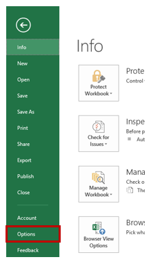
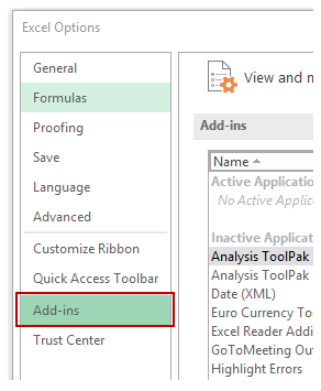
From the dialog box for options in Excel, locate the navigation pane and click Add-ins

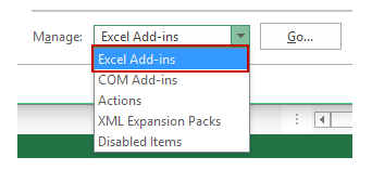
• From drop down menu for manage, choose Excel Add-ins, then Go.

• Choose the Analysis Toolpak from the dialog box for Add-ins and then OK

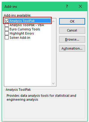
Analysis Toolpak installation will take place and then you will be able to use the Toolpak under the tab for Data.

Data Analysis Toolpak to make a histogram

After enabling Analysis Toolpak, it will give you the ability to make a histogram.

Given this set of data for 40 students and their scores for a particular course, of which the maximum mark is 100

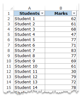
Intervals for data will have to be created if we intend to use the data to make a histogram, so that we can know the frequency of the intervals. Another name of these is bins.

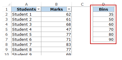
Based on the set of data, the intervals of marks are the bins.

There is the necessity to make a new column to separately show the bins.

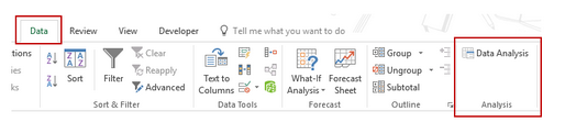
Once we have sorted out the data, we can now proceed to make the histogram.

• From the data tab, select Analysis, then Data Analysis.

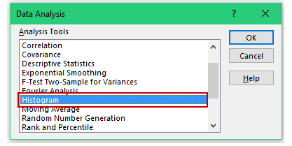
• In the list, click on Histogram, from the dialog box for Data Analysis.

• Select OK.

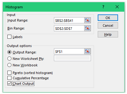
• From the dialog box for Histogram

  • Highlight the range of input (every of the students’ marks)

  • Highlight the range for Bin

  • Ensure that the checkbox for labels is not checked (you can however check it if you have data selection labels)

  • Select new workbook or worksheet if you want your chart on a new one or indicate the Output Range if you want the chart on same page.

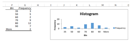
  • Click on Chart Output, then OK.

Using the function known as ‘Frequency’ to make a Histogram

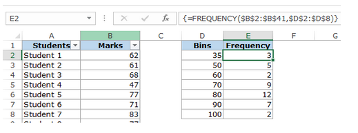
You will need to use formulas with the ‘Frequency’ function, if you want a dynamic histogram.

After getting your data and your bins, the formula you will require is:

=FREQUENCY(range of the marks, range of bins).

• Highlight every cell next to the bin.

• Use the F2 button so that the E2 cell can be in the mode for editing.

• Put in formula for Frequency shown above.

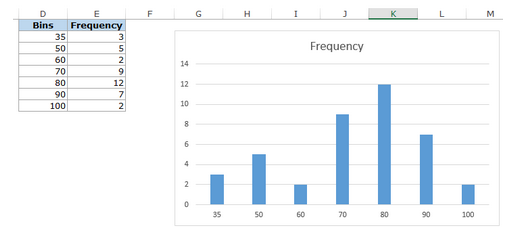
• Press Ctrl+Shift+Enter.