Why Do It?

 

Excel is all about numbers, and learning how to use numbers in Excel is essential. There are five methods you can use to look up number values in excel. These include SUMPRODUCT, SUMIF, AGGREGATE, LOOKUP and a combination of INDEX & MATCH.

This is helpful when you want to look up sales for a certain month, a balance for a customer, a price for a product, or production for a certain day.

As long as the return value is numeric, any of these formulas will work.

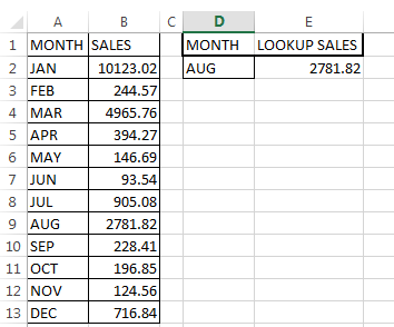
For example, we’ll look up sales values for the month of August

 

 

Using SUMPRODUCT

Syntax = SUMPRODUCT(Array1,Array2,…………,Array30)

Multiplies parallel values in matching arrays and returns sum of their products.

Arrays must be of equal size and cannot be a mix of columns and rows

Treats non-numeric values as zero

 

How it works

=SUMPRODUCT((A2:A13=D2)*(B2:B13))

 

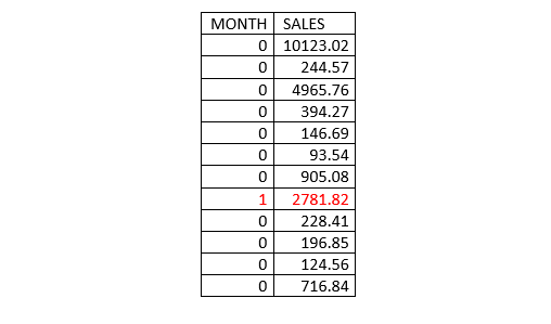
(A2:A13=D2) Returns array of TRUE/FALSE which SUMPRODUCT converts into 1/0

(B2:B13)         Returns an array of sales values

The sum of the products of above two arrays equals to sales for the suggested month

Using SUMIF

Syntax =SUMIF(criteria range, criteria, [sum range])

Sums values in a range that meet a certain criterion

It can only sum a range that is up to 255 characters

It accepts Wildcards in the criterion argument

Sum range is optional, thus, when omitted SUMIF sums the criteria range

 

How It Works

=SUMIF(A2:A13,D2,B2:B10)

 

Sums the sales for the month of August

 

Using AGGREGATE

Can either be in a Reference form or Array form

Syntax for Reference =AGGREGATE(function_num, options, ref1, [ref2], …)

Syntax for Array         =AGGREGATE(function_num, options, array, [k])

 

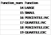
Function_num a number between 1 and 19 that determines which function to use. Function 1 to 13 use reference form

 

While 14 to 19 use array form

 

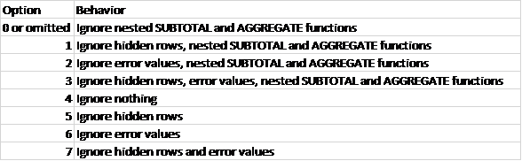
Options a number between 0 and 7 that determines which values to ignore during evaluation

 

It returns a #VALUE! Error if a required 2^nd Ref argument is not provided

Works well with data in columns or in vertical ranges

 

How It Works

=AGGREGATE(14,7,B2:B13/(A2:A13=D2),1)

 

We are using an array function (number 14—LARGE) and Option 7 which ignores hidden rows and error values

B2:B13 returns our sales values in an array

(A2:A13=D2) Returns array of TRUE/FALSE which AGGREGATE converts into 1/0

By dividing our sales values array (B2:B13) with an array of 1/0 we get an array of errors (where the divisor is zero) and Sales value (where divisor is 1)

{#DIV/0!;#DIV/0!;#DIV/0!;#DIV/0!;#DIV/0!;#DIV/0!;#DIV/0!;2781.82;#DIV/0!;#DIV/0!;#DIV/0!;#DIV/0!}

Since we choose Option 7 which ignores hidden rows and error values, LARGE function returns our sales value

 

Using LOOKUP

Looks up a value in a single row or column and finds a value from the same position in a second row or column.

syntax =LOOKUP( value, Lookup_range, [Result_range] )

 

Value—The Search value

Lookup_range—A single row or single column where the LOOKUP function searches for the value. NB: Data should be sorted in ascending order

Result_range—an Optional single row or single column of data that contains the value to be returned. NB: Must be same size as the Lookup_range.

If LOOKUP can't find a value in the Lookup_range, it returns the position of the largest/last value in the Lookup_range array that is less than or equal to the value.

The LOOKUP function then uses this position to return the value from the same position in the Result_range.

 

How It Works

=LOOKUP(1,1/(A2:A13=D2),B2:B13)

 

(A2:A13=D2) Returns array of TRUE/FALSE which LOOKUP converts into 1/0

1/(A2:A13=D2) Returns an array of Errors (#DIV/0!) where the divisor is 0 and 1 where the divisor is 1.

{#DIV/0!;#DIV/0!;#DIV/0!;#DIV/0!;#DIV/0!;#DIV/0!;#DIV/0!;1;#DIV/0!;#DIV/0!;#DIV/0!;#DIV/0!}

• LOOKUP finds the position of 1 and uses this position to returns the value from the sales value range

 

Using INDEX & MATCH

INDEX

Returns a value in a range given the row or column position. Value in the cell at the intersection of the given row and column

If row and column position is set to 0, INDEX returns an array of values for the selected range.

Can take an array format (most popular) or Reference format

Array format Syntax = INDEX( array, row_num, [col_num] )

Reference format Syntax = INDEX( range, row_num, [col_num], [area_num] )

Array—range of cells or an array constant

row_num—the row number/position in the selected array from which to return a value

col_num—the optional column number/position in the selected array from which to return a value

 

MATCH

Searches for a value in an array and returns its relative position (not the value itself) within the array.

Syntax =MATCH(lookup_value, lookup_array, [match_type])

lookup_value—the value you want to return the position of

lookup_array—the array within which to search for the value

match_type—optional numbers between -1 and 1 that specifies how excel searches for the lookup_value in the lookup_array. Default value is 1.

If no match is found, MATCH function will return the position of the last value in the array

MATCH function does not return the position of an error or blank value

 

How It Works

=INDEX(B2:B13,MATCH(D2,A2:A13,0))

 

MATCH(D2,A2:A13,0) Returns the relative position of the Month August in the array of months

INDEX(B2:B13 Returns the sales figure given the row number by the MATCH function.