We often have sheets with similar tables and with similar layout.

How to VLOOKUP from Tables in different sheets in Excel

We often have sheets with similar tables and with similar layout. They may represent months, quarters, years, or other similar sections. In this tutorial we will learn how we can use the Excel’s INDIRECT function to change the lookup table in our formulas, based on the choice we made. 

So as usual we will start with an example. We have three sheets in our sample file – Apr 17, May -17 and Summary. The first two sheets contain the tables and the last one is the summary sheet that is where we fetch the data.

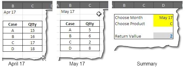
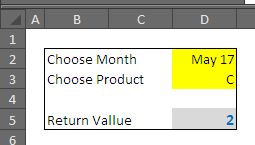
We can see that summary sheet has option to select the month and the product. In turn it gives the quantity against it. The formula we will be using is INDIRECT() with VLOOKUP(). INDIRECT will be used to provide the second argument of the VLOOKUP() function.

The syntax of INDIRECT function:

The function has following syntax:

INDIRECT(ref_text, [a1])

It is the first argument where we manipulate the information to get the desired result. All the information need to reach the correct table is present here. The second argument just defines the type of referencing. Excel has two types of referencing – A1 and R1C1. We will take up the default option and will remain them untouched.

Understanding the first argument – how to put dynamic reference in it

Let’s start by referring to the table in Apr 17.  When the table is selected the range looks like:

 Apr 17 is to be selected from the Drop down menu that is present in cell D2 in summary sheet. But before this we need to put the singles quotes before and after it. So it will become:

“’”&D2&”’!”

This way we have make the reference dynamic, but still we need to enter the range of the table:

“’”&D2&”’!”&”B4:C7”

This completely represents the reference 'Apr 17'!B4:C7.

Setting up the VLOOKUP() Formula:

The Syntax of the VLOOKUP() is not new, it takes following arguments.

VLOOKUP(lookup_value, table_array, col_index_num, [range_lookup])

The lookup_value is present in cell D3, that takes up the first argument of the formula.

VLOOKUP(D3, table_array, col_index_num, [range_lookup])

The second argument is where we  put the referencing done with INDIRECT function, the column index is 2^nd i.e. the second column and we want Exact match for our lookup:

=VLOOKUP(D3,INDIRECT("'"&D2&"'!"&"B4:C7”),2,0)

The final layout looks like:

Thus with a simple INDIRECT formula we have freedom of selecting table on different worksheets.