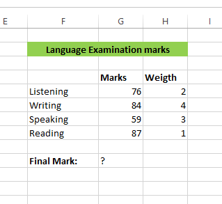
How To Calculate Weighted Average In Excel

The average value of number of cells or a data range in Excel can easily be calculated using �AVERAGE�() formula. However, there are instances that you have to calculate weighted average in order to give a better meaning to the average value. Weighted average simply means that some cells or values have more weight or priority than other cells or values.
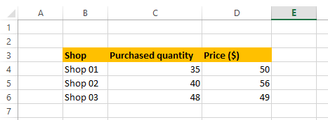
See the following example to understand the concept of weighted average. Let’s think that you want to calculate average price of an item purchased from different shops. The quantities of the item from each shop is also different.
The weighted average can be calculated by developing a simple formula following its mathematical definition.
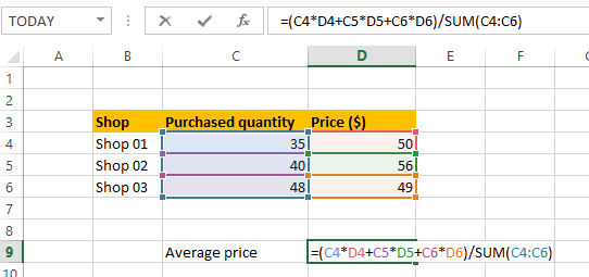
Average price = (35x50 + 40x56 + 48x49) / (35+40+48)
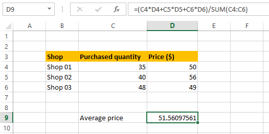
In excel, Average price = (C4*D4+C5*D5+C6*D6)/�SUM�(C4:C6)

But when there is a large number of data, typing this kind of formula would not be practical or possible. Therefore the following method can be used for any data set (large or small) to calculate the weighted average.
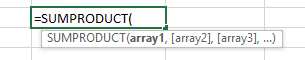
The method is based on the formula �SUMPRODUCT�() which uses the same mathematical definition for the calculation of weighted average. �SUMPRODUCT�() can have any number of arguments, though we would need only two here.
The formula for the weighted average have two parts.
Weighted average = Sum product / Sum of weights
-
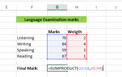
Go to the answer cell and start by typing = sign. Get �SUMPRODUCT�() formula, then add arguments to the formula. Select the cell ranges (cells, columns or rows) that you want to get sum product.
-
The first data range is marks (G5:G8) and the second is weights (H5:H8).
-
Then divide the sum product by sum of weight.
-
Press enter to get the weighted average mark.
This method is the most convenient way of calculating the weighted average, therefore wiring the long formula like in the first example, is not necessary.

Related Tutorials
Conditional Formatting is a widely used tool of Excel that provides pre-determined formatting to be applied to a cell or range of cells. The formatting may depend on the ...
INDIRECT Function yields a reference to a range. The range being referred can be a named range, a range of cells or can be a cell.

This new function allow to add handwritten equations to text, so you can add mathematical equations more easily to excel documents. The sketches of the equations can b...


Latest
-
Understanding How HYPERLINK Works In Excel
Excel has a built in function to create hyperlinks &...
-
Understanding how MS Excel Query Works
“Query” in MS Excel has same meaning as ...
-
An Introduction To Excel Power Map
Our today’s post is about “Power Map&rdq...
-
Using Pivot Charts For Displaying Data
Conventional charts are mostly used for displaying r...
-
Using “Calculated Items” For Analyzing A Pivot Table
In our last post, we explored how to use calculated ...