Conditional Formatting in Excel

Conditional Formatting is a widely used tool of Excel that provides pre-determined formatting to be applied to a cell or range of cells. The formatting may depend on the cell value or the content of it. When the cell meets the requirements of the condition, the set formats will be applied to each cell in the range.
Conditional formatting can be accessed from the ‘Home’ tab.
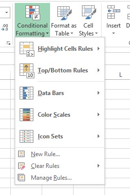
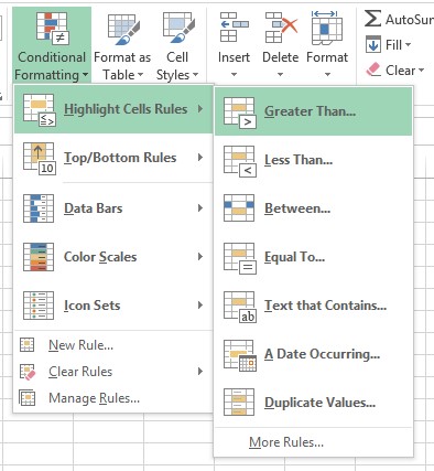
Conditional Options
The following options are available in the drop-down menu. Which can be used to format cells with numerical values, dates, text contents, find duplicates, identify variances in a range of values and other various uses.
Create a conditional formatting rule
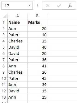
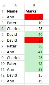
Let’s say that you want to find marks greater than 25 from the following table.
This can be easily done by applying conditional formatting.
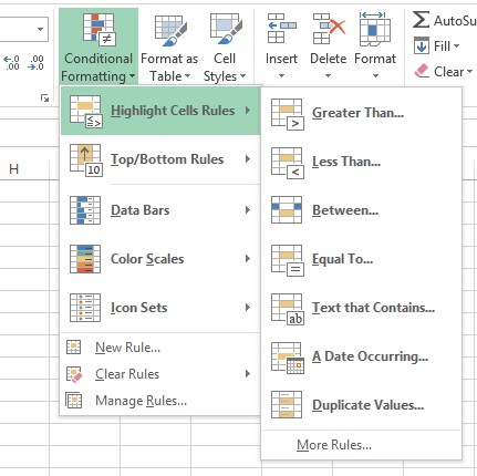
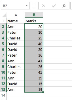
1- Select the data range that you want to be evaluated
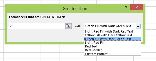
2- Go to ‘Conditional Formatting’ > Highlight cell values > Greater than..
3- Enter the pass mark and Formatting to be applied.
4- The result will be shown as follows
Also note that multiple conditional rules can also be applied.
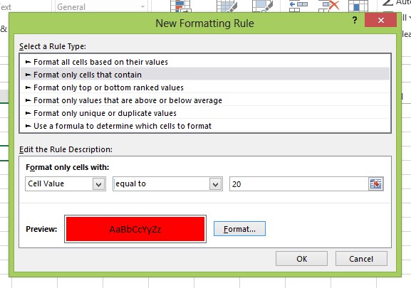
5- Again select the data range you want to be evaluated.
6- Go to ‘Conditional Formatting’ > New rule, and do the changes as required.
7- For the above requirements, following result is added to the original formatting.
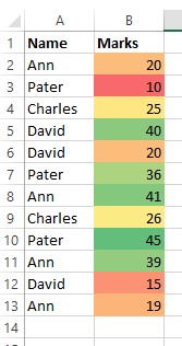
Create a conditional formatting rule 2 (applying color scale bars)
Depending on the values of the data range, a color scale can be easily given. Which would depend on the value of the cell, so the data can be visually interpreted. See the following example that we have applied color range to a data table.
To enable this option go to ‘Conditional Formatting’ > Color scales and then select and customize the color bars as you want.
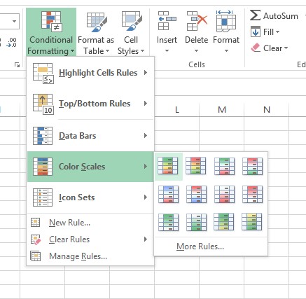
The following result is obtained for the above set conditions.

Related Tutorials

The COUNTA function is usually used for counting the non-empty cells in a given cell range.
INDIRECT Function yields a reference to a range. The range being referred can be a named range, a range of cells or can be a cell.

Format numbers according to the Indian number formatting so that 100,000 displays as 1,00,000


Latest
-
Understanding How HYPERLINK Works In Excel
Excel has a built in function to create hyperlinks &...
-
Understanding how MS Excel Query Works
“Query” in MS Excel has same meaning as ...
-
An Introduction To Excel Power Map
Our today’s post is about “Power Map&rdq...
-
Using Pivot Charts For Displaying Data
Conventional charts are mostly used for displaying r...
-
Using “Calculated Items” For Analyzing A Pivot Table
In our last post, we explored how to use calculated ...