Why do it?

Learning ways to count in Excel can save you time. Counting values in Excel using criteria is common in day to day business. For example; counting the number of failed products, overdue orders, staff in a certain department etc.

There are three methods that can be used to do this kind of count; COUNTIF, DSUM and SUMPRODUCT.

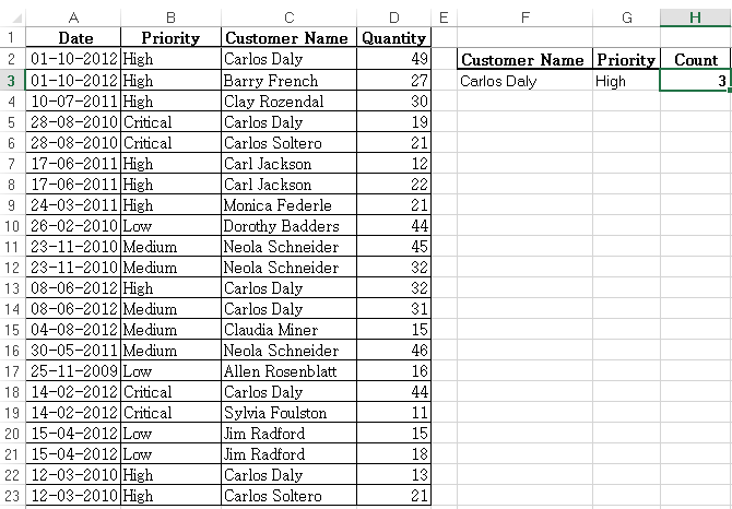
For example, Count all orders from Carlos Daly whose priority was High?

Using COUNTIFS

• Syntax =COUNTIFS(criteria_rng 1, criteria1, [criteria_rng2, criteria2]…)

• Returns the count if criteria are met

• Criteria range 1 and Criteria 1 are mandatory. Additional criteria ranges and criteria are optional to a maximum of 127 range & criteria pairs

• All ranges should be of same length otherwise formula returns #VALUE error

How It Works;

=COUNTIFS(C2:C23,F3,B2:B23,G3)=3

The formula evaluates each row at a time. If all the cells meet their associated criteria, the count increases by 1 and moves to the next row until all of the rows have been evaluated. If one cell does not meet the criteria, the formula will not increment the count

Using DSUM

• Syntax = DCOUNT(Database, Field, Criteria)

• Database—this is all data inclusive of header rows. Data area should be structured in a way that Each Row is a Record, Each Column is a Field & Top rows contain headers that identify the fields

• Field –this is a column that holds ONE particular item of data e.g. Dates or Names. Can be omitted and still count records that meet all criteria.

• Criteria—this is section in the Worksheet (apart from the database) which holds Criteria. Criteria Area should be set in such a way that for every header, there is a cell below it where you enter the criterion to be met. The area MUST NOT include any Blank rows or Columns

How It Works;

=DCOUNT(A1:D23,,F2:G3)=3

The formula counts the occurrences in the database “A1:D23” where “Customer Name = Carols Daly” and “Priority = High”

Using SUMPRODUCT

• Syntax = SUMPRODUCT(Array1,Array2,…………,Array30)

• Multiplies parallel values in matching arrays and returns sum of their products

• Arrays must be of equal size and cannot be a mix of columns and rows

• Treats non-numeric values as zero

How it Works:

=SUMPRODUCT((C2:C23=F3)*(B2:B23=G3))=3

(C2:C23=F3) Returns array of TRUE/FALSE depending on the customer name. SUMPRODUCT converts this Boolean array into its numeric equivalent of 1/0

(B2:B23=G3) Returns array of TRUE/FALSE depending on the order priority. SUMPRODUCT converts this Boolean array into its numeric equivalent of 1/0

SUMPRODUCT then multiplies the values of the two arrays and sums up the product

=SUMPRODUCT({1;0;0;1;0;0;0;0;0;0;0;1;1;0;0;0;1;0;0;0;1;0}*{1;1;1;0;0;1;1;1;0;0;0;1;0;0;0;0;0;0;0;0;1;1})