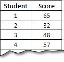
Let’s assume you are a math’s teacher interested in finding the average of the math’s score of last five students – he is interested in finding why they are performing poor. How will he proceed?

In Excel we have conditional averaging formula called AVERAGEIF() or for more then one criteria we have AVERAGEIFS(). But these are not array formulas by default and need helper columns to perform averaging.

In this post, we will learn the default solution to this problem that is AVERAGEIF() from Excel and a an array formula (that we will produce) to do it without any helper column.

So let’s start with the data.

The data:

We have created data using RANDBETWEEN () function. The data is present in the range B2:C21.

Solution # 01 – Using the default AVERAGEIF() formula.

We can use the built in AVERAGEIF() formula to achieve the task, but before this we need to setup a helper column. We need to put the data in ascending order to get the list sorted and then we will average the first five values (the smallest ones) in the list.

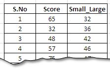
The formula used in the Small_Large column: =SMALL($C$3:$C$21,ROW(A1))

With this formula, as we drag it down, we have the sorted list of numbers. As we drag down the formula, the second argument of the formula changes accordingly due to relative referencing.

The result will be obtained and displayed in the following form:

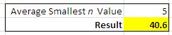
And the formula used for averaging here is: =AVERAGEIF($B$3:$B$21,"<="&$G$2,$D$3:$D$21)

In this formula the second term, "<="&$G$2 sets the criteria for numbers to be averaged by making sure that they are less then or equal to given n numbers – here 5. This means that only first 5 smallest numbers will be averaged.

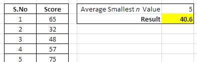
Solution # 02 – Using array formula to get the solution:

For this case we will use the following formula:

=AVERAGE(SMALL(C3:C21,ROW(INDIRECT("A1:A"&F2))))

…with Ctrl+Shfit+Enter.

How this formula does works?

Lets start breaking this formula up in to components. We start from the very inner bracket i.e. INDIRECT("A1:A"&F2). This part produces the array that has to be dynamic and is to be feed to ROW() function. You can see that we have an option to enter the n values to be averaged. For these,  we have to have the array from 1…n i.e. the array need to be dynamic. This is done by using the INDIRECT() function that takes value from cell F2.

If the value is 5 it will return A1:A5, if the value is 8 it will return A1:A8. And that will be feed to ROW()

When the value is feed to row it will produce an array: {1,2,3,4,5} that will act as second argument of the function SMALL(). With this arrangement, it will return a corresponding five (or n) smallest  values: {{32,36,42,46,47} and the AVERAGE() function will average it.

..and off course you need to execute this formula with CSE.

This was all about this post, please download the file form this link.