Introduction To Slicers In Excel 2010

You must have used filters in Excel! Whether you are using a table or have a list, whenever you have data and want to search for certain information, filters are there for you. Slicers are simply visual filters! Unlike with filters, where you have to select a header row, insert them first, scroll and select them first and then filter – slicer let you select from a visual list of options that you can select from and filter.
Slicers in Excel 2010 depends on a background pivot table that has to be added first, and then slicers be inserted. From Excel 2013, we can have standalone slicers in our sheets.
In this short post, we will learn how to insert a slicers, how to use them and some tips and tricks, related to them.
Filters Vs Slicers
Conventionally you have to put your cursor first in the header row and then go to Data > Select Filter and then filter appears in the header row….
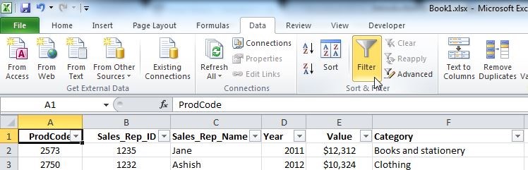
Once you have selected and applied filters, you can choose from the set of options available.
On the other hand you have to insert a pivot table first to apply the Slicers. For Excel 2010, you need to go to Insert menu, Insert a Pivot Table first.
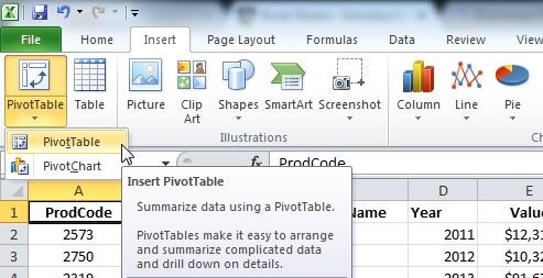
Once you have a Pivot table in place, you can apply Slicers…
-
From the Pivot Table Tab, select Slicers > Insert Slicers
-
Inserting Slicers will show you a dialogue box with All Available Fields in the Table, Select one you need to use.
-
Once done, you will see following windows to select from…
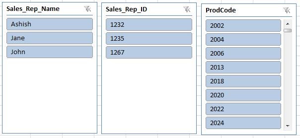
And the pivot table will start filtering based on the selection from these lists.
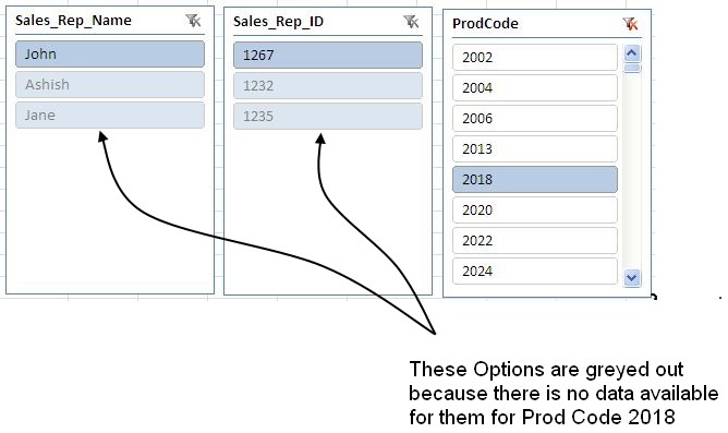
Grayed out options
A slicer may have grayed out options if they are not available for selection.
Using Slicer
How can we use it? Just like we used filters! Let’s assume that we want to find the total sales for “Alcohol” in year 2011. What we need to do is:
-
For Category select Alcohol
-
For Year select 2011
-
The pivot table should show total sales and ProdCode wise breakup of the data.
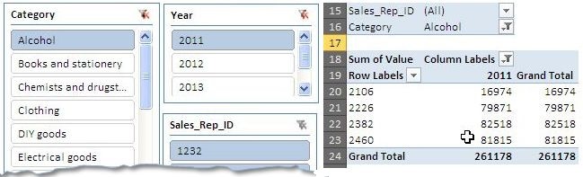
The total sales for Year 2011 for Alcohol are $261178. But we can still drill down. Select few more of the fields form the slicers and you find much more about the data.
Creating Charts that work on Slicers:
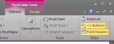
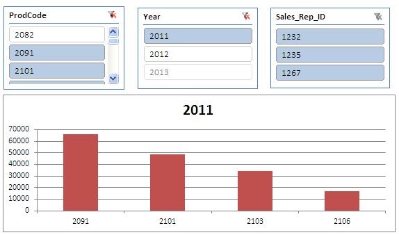
Since the pivot tables is basis for Slicers, we can also add pivot charts that work on them. You can go to Pivot Table options and insert a Pivot Chart:
Once inserted you can format it to your taste and enjoy filtering it using Slicers. You can always select more options at once by pressing Ctrl Key and then selecting.
This is all for this post. Please download the workbook and see how things are working.

Related Tutorials
Conventional charts are mostly used for displaying rather “static” data from excel sheets – i.e. if you have a table where you have manually entered ...

Suppose you want to randomize a list, for this you have to have a list of random (or shuffled) numbers, which can be used to randomize the list you want.
Consider a case where you have a table like below and want to fetch the data for a single month.


Latest
-
Understanding How HYPERLINK Works In Excel
Excel has a built in function to create hyperlinks &...
-
Understanding how MS Excel Query Works
“Query” in MS Excel has same meaning as ...
-
An Introduction To Excel Power Map
Our today’s post is about “Power Map&rdq...
-
Using Pivot Charts For Displaying Data
Conventional charts are mostly used for displaying r...
-
Using “Calculated Items” For Analyzing A Pivot Table
In our last post, we explored how to use calculated ...